


What is Würstchen?
Würstchen is a diffusion model, and its text conditional component operates in a highly compressed latent space of images. Why is this important? Compressing data can reduce computational costs for both training and inference by orders of magnitude. Training on 1024×1024 images is much more expensive than training on 32×32. Other works typically use relatively small compressions ranging from 4x to 8x spatial compression. Würstchen takes this to the extreme. The innovative design achieves 42 times more space compression! This has never been seen before, as common methods cannot faithfully reconstruct detailed images after 16x spatial compression. Würstchen employs two stages of compression called Stage A and Stage B. Stage A is a VQGAN and stage B is a diffuse autoencoder (details are provided in the paper). Stages A and B are collectively called the decoder because they decode the compressed image back into pixel space. The third model, Stage C, is trained in its highly compressed latent space. This training requires some of the compute used by today’s best-performing models, but also enables cheaper and faster inference. Stage C is called the pre-stage.

Why a separate text-to-image model?
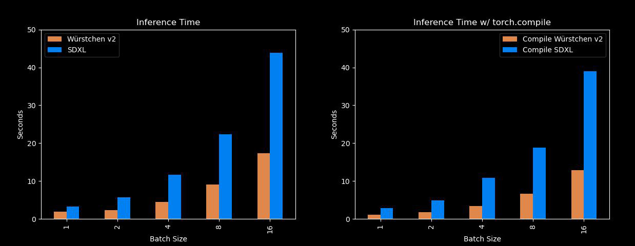
Well, this is pretty fast and efficient. Würstchen’s biggest advantage lies in the fact that it can generate images much faster than models such as Stable Diffusion XL, while also using significantly less memory. So for those who don’t have an A100, this will come in handy. Below is a comparison with SDXL at various batch sizes.
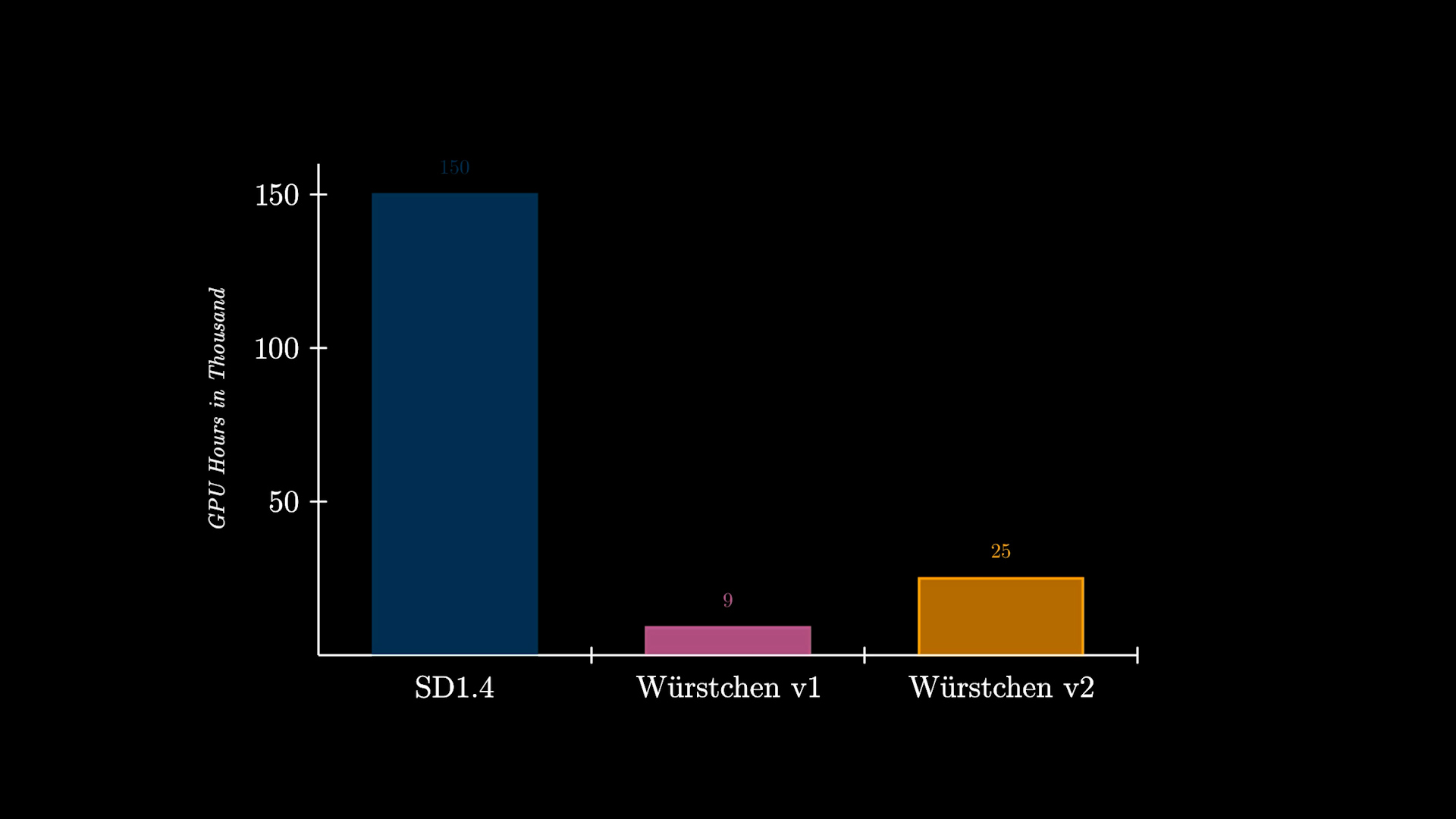
In addition to that, another big advantage of Würschen is reduced training costs. Würstchen v1 ran at 512×512 and required only 9,000 hours of GPU time to train. Comparing this to the 150,000 GPU hours spent on Stable Diffusion 1.4 suggests that this 16x cost reduction not only benefits researchers when conducting new experiments, but also opens the door for more organizations to train such models. Würstchen v2 used 24,602 GPU hours. Even when the resolution goes up to 1536, it is still 6x cheaper than SD1.4, which was only trained on 512×512.
A detailed instructional video is also available here.
How to use Würstchen?
You can try it out using the demo here.
Otherwise, models are available from the Diffuser Library, so you can use a familiar interface. For example, here’s how to perform inference using AutoPipeline:
import torch
from diffuser import AutoPipelineForText2Image
from Diffuser.Pipeline.Wurstchen import DEFAULT_STAGE_C_TIMESTEPS pipeline = AutoPipelineForText2Image.from_pretrained(“Warp Eye/Verstchen”torch_dtype=torch.float16).to(“Cuda”) caption = “Anthropomorphic cat dressed as a firefighter”
image = pipeline( caption, height =1024width =1536prior_timesteps=DEFAULT_STAGE_C_TIMESTEPS, prior_guidance_scale=4.0number of images per prompt =4,).image

What image sizes does Würschen support?
Würstchen was trained on image resolutions from 1024×1024 to 1536×1536. Resolutions such as 1024×2048 may also provide good output. Please try it. We also observed that Prior (stage C) adapts to the new resolution very quickly. Therefore, fine-tuning at 2048×2048 should be less computationally expensive.

model on hub
All checkpoints can also be found on the Huggingface Hub. There are multiple checkpoints, as well as weights for future demos and models. There are currently three checkpoints available for Prior and one checkpoint for Decoder. See the documentation that describes checkpoints and the documentation that describes the overview and availability of various previous models.
Diffuser integration
Since Würstchen is fully integrated into the diffuser, it automatically provides a wide range of out-of-the-box functions and optimizations. These include:
As explained below, automatic use of PyTorch 2 SDPA increased alertness. 2. Support for xFormers flush attention implementation if you need to move unused components to the CPU using PyTorch 1.x instead of model offloading. This saves memory with negligible performance impact. Sequential CPU offloading for situations where memory is at a premium. Memory usage is minimal, but inference is slower. Instant weighting using the Compel library. Support for mps devices on Apple Silicon Macs. Use a generator to increase reproducibility. Sensible defaults for inference produce high-quality results in most situations. Of course, you can fine-tune all parameters to your needs.
Optimization Technique 1: Flash Attention
Starting with version 2.0, PyTorch has integrated a highly optimized and resource-friendly version of the attention mechanism called torch.nn.function.scaled_dot_product_attention (SDPA). Depending on the nature of the input, this function utilizes several fundamental optimizations. Its performance and memory efficiency outperform traditional attention models. Notably, the SDPA feature reflects the characteristics of flash attention technology, as highlighted in the research paper “Fast and Memory-Efficient Exact Attending with IO-Awareness” authored by Dao and his team.
If you are using Diffuser with PyTorch 2.0 or later versions and have access to SDPA features, these extensions will be applied automatically. Get started by setting up torch 2.0 or later versions using the official guidelines.
image = pipeline(caption, height =1024width =1536prior_timesteps=DEFAULT_STAGE_C_TIMESTEPS, prior_guidance_scale=4.0number of images per prompt =4).image
To learn more about how diffusers utilize SDPA, check out our documentation.
If you are using a version of Pytorch earlier than 2.0, you can still achieve memory-efficient attention using the xFormers library.
Pipeline.enable_xformers_memory_efficient_attention()
Optimization technique 2: Torch compilation
If you want even more performance, you can use torch.compile. For maximum performance, it is best to apply it to both the previous model and the main model of the decoder.
Pipeline.prior_prior = torch.compile(pipeline.prior_prior , mode=“Reducing overhead”full graph =truth) pipeline.decoder = torch.compile(pipeline.decoder, mode=“Reducing overhead”full graph =truth)
Note that during model compilation, the first inference step takes a long time (up to 2 minutes). You can then perform inference as usual.
image = pipeline(caption, height =1024width=1536prior_timesteps=DEFAULT_STAGE_C_TIMESTEPS, prior_guidance_scale=4.0number of images per prompt =4).image
And the good news is that this compilation is a one-time run. You can then experience consistently fast inference at the same image resolution. The initial investment in compilation is quickly offset by subsequent speed benefits. If you want to learn more about torch.compile and its nuances, check out the official documentation.
How was the model trained?
The ability to train this model was only possible through the computing resources provided by Stability AI. We would like to give a special thanks to Stability for giving us the opportunity to make this type of research available to even more people.
resource
For more information about this model, please refer to the official diffuser documentation. All checkpoints are located at the hub. You can try the demo here. If you’d like to discuss upcoming projects or contribute your own ideas, please join us on Discord. Training code and more can be found in the official GitHub repository.
